
Motivation
The Adafactor optimizer, in my experience, can provide much better convergence when fine-tuning the T5 v1.1 and mT5[1] pre-trained models. However, I encountered problems when using a custom learning rate scheduler with the Adafactor implementation from the huggingface/transformer library. I combed through the paper and the source code to find and fix the cause of the problem, which turned into a tiny contribution to the library.
To further squeeze value from the time I’ve invested, I wrote this post to introduce the key ideas of the Adafactor optimizer and analyze the corresponding chunk of code in the huggingface/transformer implementation (which was taken from the fairseq library). Working examples as Kaggle notebooks are also provided: T5 v1.1 and mT5.
(Notes: For the original T5 pre-trained models[2], which were pre-trained with a mixture of unsupervised and supervised objectives, Adam or AdamW optimizers are enough to get good results.)
Overview
The popular Adam[3] optimizer keeps two additional values for each parameter. One stores the momentum; one stores the exponentially smoothed squared gradients. Therefore, the memory requirement is tripled comparing to the vanilla SGD optimizer. Adafactor dramatically reduces this requirement (more than half) while retaining comparable performance (tested on the WMT ’14 En→De translation task with the classic transformer seq2seq architecture).
The authors of Adafactor firstly propose to replace the full smoothed squared gradients matrix with a low-rank approximation. This reduces the memory requirements for the squared gradients from O(nm) to O(n+m).
Secondly, Adafactor removes momentum entirely. This causes some training instability. The authors think that the out-of-date second-moment accumulator (the exponential smoothing of the squared gradients) might be the cause. By increasing the decay rate with time (new values have higher importance) and clipping the gradient update, Adafactor can converge normally even without momentum.
Finally, Adafactor multiplies the learning rate by the scale of the parameters (this is called “relative step size”). The authors showed that training with relative step sizes provides more robustness to differently scaled embedding parameters.
Factored Second Moment Estimation
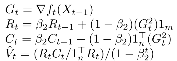
Adafactor refactor the exponential moving average of squared gradients $V \in \mathbb{R}^{n \times m}$ to $RS$, where $R \in \mathbb{R}^{n \times 1}$ and $S \in \mathbb{R}^{1 \times m}$. It has an analytic solution for minimizing the I-divergence (generalized Kullback-Leibler divergence):
The solution only requires us to store the moving averages of the row sums and the column sums:
Alg 1: The low-rank approximation of V
Looking at the corresponding part in the implementation, here’s the part that update the moving average of the row and column sums:
exp_avg_sq_row.mul_(beta2t).add_(1.0 - beta2t, update.mean(dim=-1))
exp_avg_sq_col.mul_(beta2t).add_(1.0 - beta2t, update.mean(dim=-2))
And the implementation of the analytic solution (rsqrt means the reciprocal of the square root $1/\sqrt{input}$):
@staticmethod
def _approx_sq_grad(exp_avg_sq_row, exp_avg_sq_col):
    r_factor = (exp_avg_sq_row / exp_avg_sq_row.mean(dim=-1, keepdim=True)).rsqrt_()
    c_factor = exp_avg_sq_col.rsqrt()
    return torch.mm(r_factor.unsqueeze(-1), c_factor.unsqueeze(0))
The above corresponds to $1/\hat{V}_t = 1/(R_tCt/1^\intercal_nR_t)$. The $(1 - \beta^{t}_2)$ part (a.k.a. bias correction) in Alg 1 has been removed due to a reformulation of $\beta^{t}_2$ in the latter part of the paper.
Removing Momentum
The authors demonstrated that fast decay of the second moment estimator has convergence problems, while slow decay has stability problems:
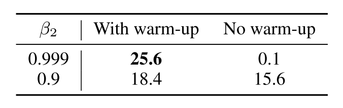
Table 1
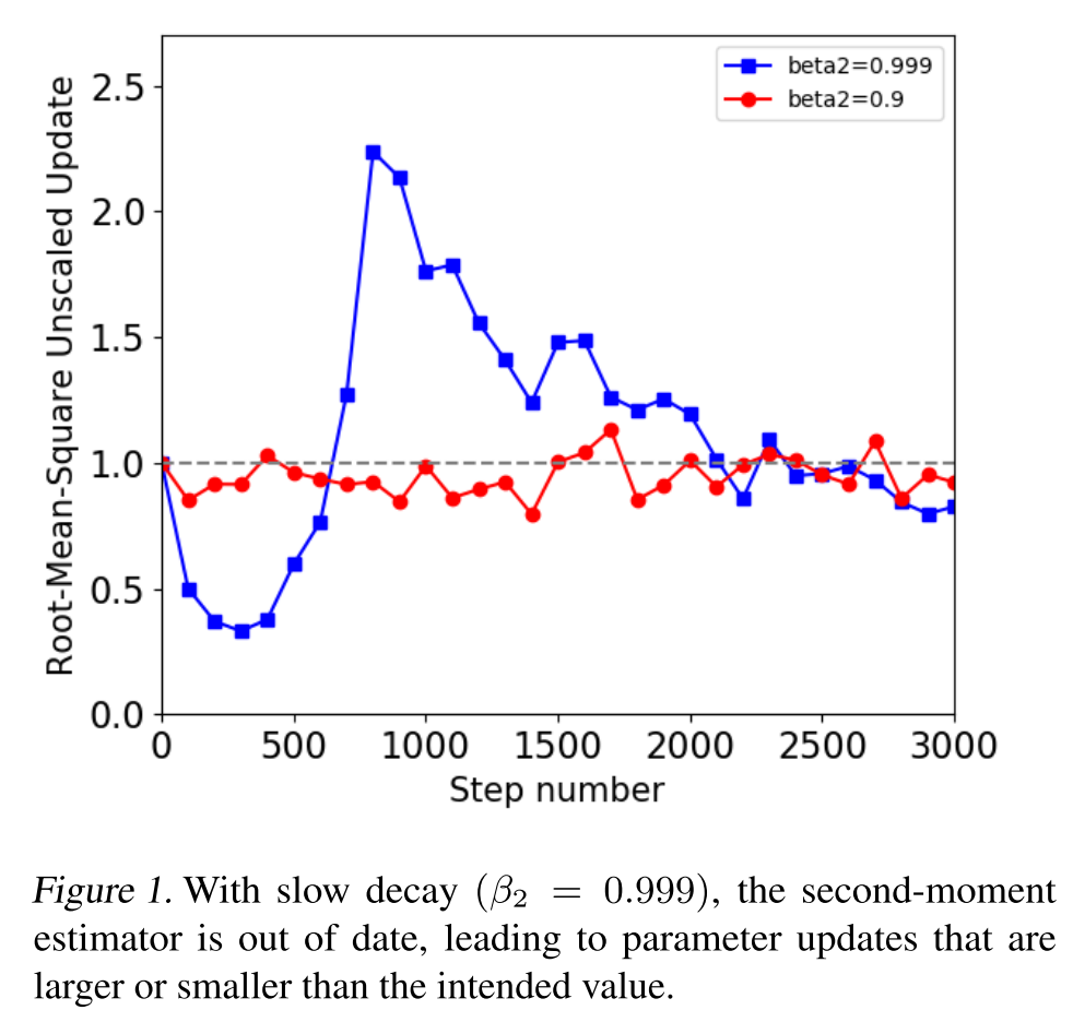
And the problem of slow decay is the larger-than-desired updates:
Update Clipping
One of the proposed solutions is to clip the update according to the root-mean-square over all parameters in a weight matrix or vector:
RMS is implemented as a static method:
@staticmethod
def _rms(tensor):
    return tensor.norm(2) / (tensor.numel() ** 0.5)
The tensor should already be unscaled (i.e., $\frac{g_{xt}}{\sqrt{v_{xt}}}$). The .norm(2) calculates the root sum squared, and .numel() ** 0.5 convert it to the root mean squared.
The update then is clipped accordingly to a threshold $d$:
update.div_((self._rms(update) / group["clip_threshold"]).clamp_(min=1.0))
update.mul_(lr)
It will effectively cap the unscaled update at $d$ (a horizontal line in Figure 1.).
Increasing Decay Parameter
Another solution is to use an increasing $\beta_2$. The proposed family of schedules is:
This can be implemented in a one-liner:
beta2t = 1.0 - math.pow(state["step"], group["decay_rate"])
Note that $\hat{\beta}_{2t}$ has been the reformulated, which eliminates the need to do bias correction.
Relative Step Size
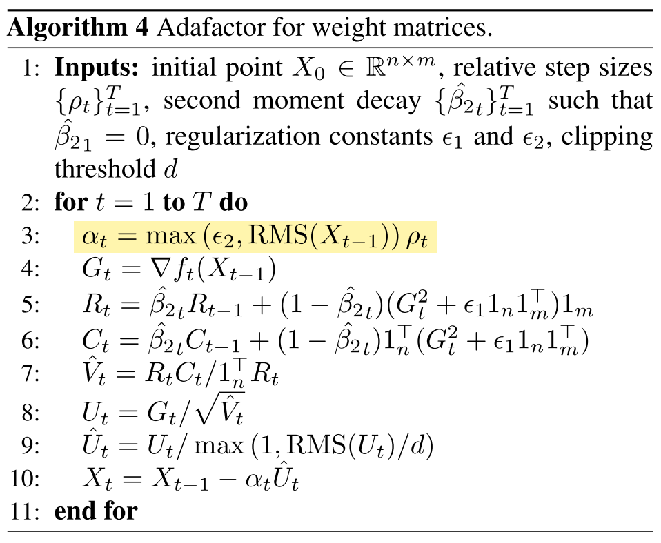
Adafactor multiplies the given learning rate by the scale of the parameters, which is defined as the root-mean-square of its components. Therefore, parameters with bigger values get bigger updates and vice versa:
The paper calls $\alpha_t$ the “absolute step size” and $\rho_t$ the “relative step size.”
The relative step size is implemented here:
if param_group["scale_parameter"]:
    param_scale = max(param_group["eps"][1], param_state["RMS"])
return param_scale * rel_step_sz
The $RMS(X_{t−1})$ notation might make you think that the RMS is calculated on the parameters of the entire model. But the RMS is in fact calculated on a single parameter tensor (a matrix or a vector). This makes sense because we want the learning rate scale to closely follow the scale of the parameters. (The p_data_fp32 below is a tensor.)
state["RMS"] = self._rms(p_data_fp32)
Now we have the complete Adafactor algorithm:
Confusing Parameter Naming
One problem of this implementation is the naming of its class parameters. There are three parameters that control the learning rate: scale_parameter, warmup_init, and relative_step. But in fact, only the first parameter — scale_parameter — implements the relative step size in the last section. The latter two only control the learning rate schedule.
With relative_step=True and warmup_init=False, the learning rate will use a simple inverse-square root decay used by the paper:
With relative_step=True and warmup_init=True, it adds a linear warmup stage to the schedule:
They are implemented in the _get_lr static method:
rel_step_sz = param_group["lr"]
if param_group["relative_step"]:
    min_step = 1e-6 * param_state["step"] if param_group["warmup_init"] else 1e-2
    rel_step_sz = min(min_step, 1.0 / math.sqrt(param_state["step"]))
As you can see, there’s nothing to do with learning rate scaling by the magnitude of the parameter.
Using Custom Learning Rate Schedule
Astute readers might already notice that when relative_step=False and warmup_init=False, the rel_step_size is simply the learning rate the user has given to the optimizer. We can use regular PyTorch learning rate schedulers to control that variable. My pull request fixed a bug that prevents the variable from being incorrectly updated by Adafactor.
Working Examples
I’ve written some code that fine-tunes T5 and mT5 models on NLI datasets using PyTorch Lightning. This is where I set up the Adafactor optimizer:
optimizer = Adafactor(
    self.model.parameters(),
    relative_step=False, warmup_init=False,
    clip_threshold=1.0, lr=self.config.learning_rate,
    scale_parameter=True
)
I used a combination of linear warmup and cosine annealing to schedule the learning rates:
scheduler = {
    'scheduler': pls.lr_schedulers.MultiStageScheduler(
        [
            pls.lr_schedulers.LinearLR(optimizer, 0.0001, lr_durations[0]),
            CosineAnnealingLR(optimizer, lr_durations[1])
        ],
        start_at_epochs=break_points
    ),
    'interval': 'step',
    'frequency': 1,
    'strict': True,
}
I’ve published a Kaggle notebook that fine-tunes the google/t5-v1_1-base model on the MultiNLI dataset and gets a competitive result. I’ve observed that my learning rate schedule performs better than the inverse-square root decay recommended by the paper.
An mT5 version that further fine-tunes an MNLI fine-tuned google/mt5-base model on a multi-lingual dataset is also available. Because of the low resource of the multi-lingual corpus, I froze the embedding matrix in this one to prevent overfitting.
References
- Xue, L., Constant, N., Roberts, A., Kale, M., Al-Rfou, R., Siddhant, A., … Raffel, C. (2020). mT5: A massively multilingual pre-trained text-to-text transformer.
- Raffel, C., Shazeer, N., Roberts, A., Lee, K., Narang, S., Matena, M., … Liu, P. J. (2019). Exploring the Limits of Transfer Learning with a Unified Text-to-Text Transformer.
- Kingma, D. P., & Ba, J. L. (2015). Adam: A method for stochastic optimization.