Introduction
NLP(Natural-language processing) is hard, partly because human is hard to understand. We need good tools to help us analyze texts. Even if the texts are eventually fed into a black box model, doing exploratory analysis is very likely to help you get a better model.
I’ve heard great things about a R package tidytext and recently decided to give it a try. The package authors also wrote a book about it and kindly released it online: Text Mining with R: A guide to text analysis within the tidy data framework, using the tidytext package and other tidy tools.
As the name suggests, tidytext aims to provide text processing capability in the *tidyverse* ecosystem. I was more familiar with data.table and its way of data manipulation, and the way tidyverse handles data had always seemed tedious to me. But after working through the book, I’ve found the syntax of *tidyverse* very elegant and intuitive. I love it! All you need is some good examples to help you learn the ropes.
Chapter 7 of the book provides a case study comparing tweet archives of the two authors. Since twitter only allows downloading the user’s own archive, it is hard for a reader without friends (i.e. me) to follow. So I found a way to download tweets of public figures and I’d like to share with you how to do it. This post also presents an example comparing tweets from Donald Trump and Barack Obama. The work flow is exactly the same as in the book.
Warning: The content of this post may seem very elementary to professionals.
R tips
-
Use Microsoft R Open if possible. It comes with the multi-threaded math library (MKL) and checkpoint package.
-
But don’t hesitate to switch to regular R if you run into trouble. Microsoft R Open can have some bizarre problems in my personal experiences. Don’t waste too much time on fixing them. Switching to regular R often solves the problem.
-
Install regular R via CRAN (Instructions for Ubuntu). Install checkpoint to ensure reproducibility (it is not a Microsoft R Open exclusive.)
-
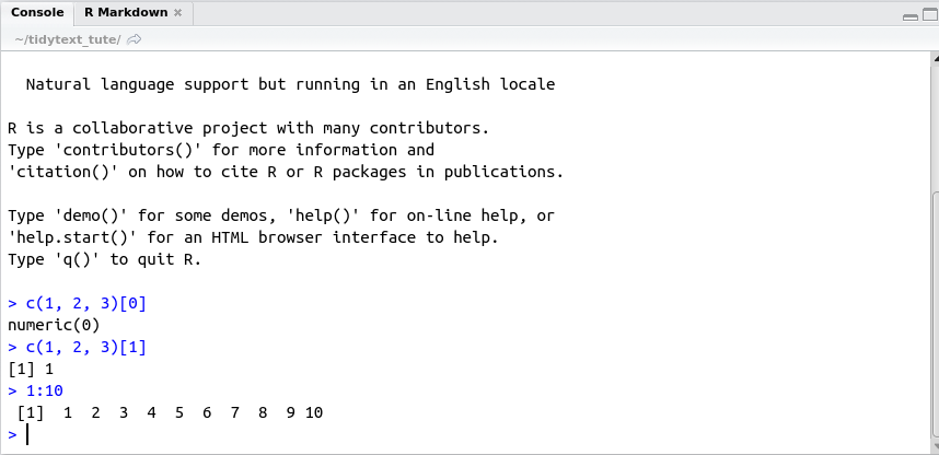
Use RStudio and make good use of its Console window. Some people hold strong feelings against R because of some of its uniqueness comparing to other major programming languages. In fact a lot of the confusion can be resolved with simple queries in the Console. Not sure whether the vector index starts from zero or one?
c(1,2,3)[1]tells you it’s one. Querying1:10tells you the result includes 10 (unlike Python).
Getting the data and distribution of tweets
First of all, follow the instruction of this article to obtain your own API key and access token, and install twitteR package: Accessing Data from Twitter API using R (part1).
You need these four variables:
consumer_key <- "FILL HERE"
consumer_secret <- "FILL HERE"
access_token <- "FILL HERE"
access_secret <- "FILL HERE"
The main access point for this post is userTimeline. It downloads at most 3200 recent tweets of a public twitter user. The default includeRts=FALSE parameter seems to remove a lot of false positives, so we’ll instead do it manually later.
setup_twitter_oauth(
    consumer_key, consumer_secret, access_token, access_secret)

trump <- userTimeline("realDonaldTrump", n=3200, includeRts=T)
obama <- userTimeline("BarackObama", n=3200, includeRts=T)
president.obama <- userTimeline("POTUS44", n=3200, includeRts=T)
Now we have tweets from @realDonaldTrump, @BarackObama and @POTUS44 as List objects. We’ll now convert them to data frames:
df.trump <- twListToDF(trump)
df.obama <- twListToDF(obama)
df.president.obama <- twListToDF(president.obama)

(The favorited, retweeted columns are specific to the owner of the access token.) We’re going to only keep columns text, favoriteCount, screenName, created and retweetCount, and filter out those rows with isRetweet=TRUE. (statusSource might be of interest in some applications.)
tweets <- bind_rows(
  df.trump %>% filter(isRetweet==F) %>%
    select(
      text, screenName, created, retweetCount, favoriteCount),
  df.obama %>% filter(isRetweet==F) %>%
    select(
      text, screenName, created, retweetCount, favoriteCount),
  df.president.obama %>% filter(isRetweet==F) %>%
    select(
      text, screenName, created, retweetCount, favoriteCount))
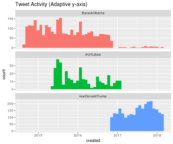
Now we plot the time distribution of the tweets:
ggplot(tweets, aes(x = created, fill = screenName)) +
  geom_histogram(
    position = "identity", bins = 50, show.legend = FALSE) +
  facet_wrap(~screenName, ncol = 1, scales = "free_y") +
  ggtitle("Tweet Activity (Adaptive y-axis)")
You could remove scales = "free_y" to have compare the absolute amount of tweets instead of relative:
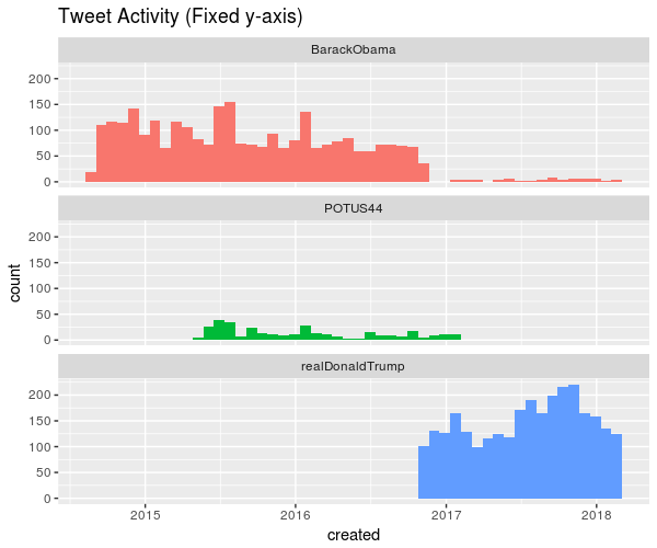
(The lack of activity of @realDonaldTrump is from the 3200-tweet restriction) We can see that as a president, Donald Trump tweets a lot more than Barack Obama did.
Word frequencies
From this point we’ll enter the world of tidyverse:
replace_reg <- "http[s]?://[A-Za-z\\d/\\.]+|&|<|>"
unnest_reg <- "([^A-Za-z_\\d#@']|'(?![A-Za-z_\\d#@]))"
tidy_tweets <- tweets %>%
filter(!str_detect(text, "^RT")) %>%
mutate(text = str_replace_all(text, replace_reg, "")) %>%
mutate(id = row_number()) %>%
unnest_tokens(
word, text, token = "regex", pattern = unnest_reg) %>%
filter(!word %in% stop_words$word, str_detect(word, "[a-z]"))
(It’s worth noting that the pattern used in unnest_tokens are for matching separators, not tokens.) Now we have the data in one-token-per-row tidy text format. We can use it to do some counting:
frequency <- tidy_tweets %>%
  group_by(screenName) %>%
  count(word, sort = TRUE) %>%
  left_join(tidy_tweets %>%
              group_by(screenName) %>%
              summarise(total = n())) %>%
  mutate(freq = n/total)

frequency.spread <- frequency %>%
  select(screenName, word, freq) %>%
  spread(screenName, freq) %>%
  arrange(desc(BarackObama), desc(realDonaldTrump))

ggplot(frequency.spread, aes(BarackObama, realDonaldTrump)) +
  geom_jitter(
    alpha = 0.1, size = 2.5, width = 0.15, height = 0.15) +
  geom_text(aes(label = word), check_overlap = TRUE, vjust = 0) +
  scale_x_log10(labels = percent_format()) +
  scale_y_log10(labels = percent_format()) +
  geom_abline(color = "red") + theme_bw()
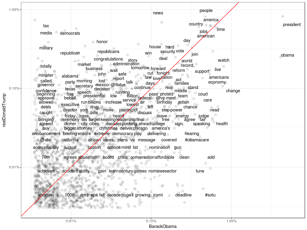
Comparison of Word Frequencies
(Because of the jitters, the text labels sometimes are far away from its corresponding data point. So far I don’t have a solution for this problem.) One observation from the above plot is the more frequent use of “republicans” , “republican”, and “democrats” by Trump.
Comparing word usage
word_ratios <- tidy_tweets %>%
  filter(screenName != "POTUS44") %>%
  filter(!str_detect(word, "^@")) %>%
  count(word, screenName) %>%
  filter(sum(n) >= 10) %>%
  ungroup() %>%
  spread(screenName, n, fill = 0) %>%
  mutate_if(is.numeric, funs((. + 1) / sum(. + 1))) %>%
  mutate(logratio = log(realDonaldTrump / BarackObama)) %>%
  arrange(desc(logratio))

word_ratios %>%
  group_by(logratio < 0) %>%
  top_n(15, abs(logratio)) %>%
  ungroup() %>%
  mutate(word = reorder(word, logratio)) %>%
  ggplot(aes(word, logratio, fill = logratio < 0)) +
  geom_col(show.legend = FALSE) +
  coord_flip() +
  ylab("log odds ratio (realDonaldTrump/BarackObama)") +
  scale_fill_discrete(name = "", labels = c("realDonaldTrump", "BarackObama"))
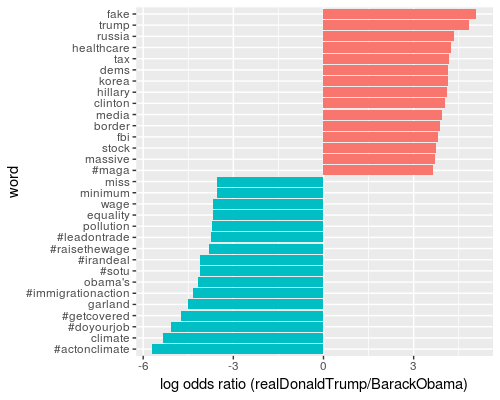
Comparison of Word Frequencies
Readers can find the dramatically different characteristics of the two presidents from the plot. But to be fair, some of the words from Obama are hashtags that are unlikely to be re-used later. Let’s see what will come up when we remove the hashtags:

Most Distinctive Words (excluding hastags)
Changes in word use
This part is more involved, so I’ll skip the source code. The idea is to fit a glm model to predict the word frequency with the relative point of time. If the coefficient of the point of time is very unlikely to be zero (low p value), we say that the frequency of this word has changed over time. We plot the words with lowest p values for each president below:
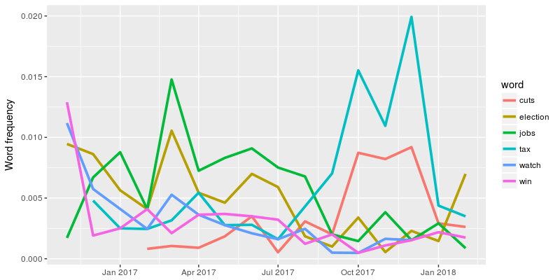
Donald Trump
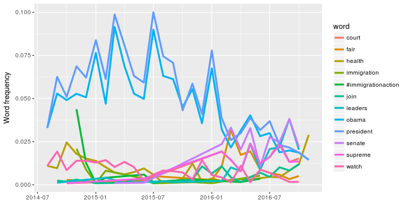
Barack Obama
For Barack Obama, only tweets from his presidency has been included because of the sparsity of the tweets in 2017 and beyond. Please check the book or the R Markdown link at the end of the post for source code and more information.
Favorites and retweets
We can count all the retweets and favorites and count which words are more likely to appear. Note it’s important to count each word only once in every tweet. We achieve this by grouping by (id, word, screenName) and summarise with a *first *function:
totals <- tweets %>%
  group_by(screenName) %>%
  summarise(total_rts = sum(retweetCount))

word_by_rts <- tidy_tweets %>%
  group_by(id, word, screenName) %>%
  summarise(rts = first(retweetCount)) %>%
  group_by(screenName, word) %>%
  summarise(retweetCount = median(rts), uses = n()) %>%
  left_join(totals) %>%
  filter(retweetCount != 0) %>%
  ungroup()

word_by_rts %>%
  filter(uses >= 5) %>%
  group_by(screenName) %>%
  top_n(10, retweetCount) %>%
  arrange(retweetCount) %>%
  ungroup() %>%
  mutate(
    word = reorder(
      paste(word, screenName, sep = "__"),
      retweetCount)) %>%
  ungroup() %>%
  ggplot(aes(word, retweetCount, fill = screenName)) +
  geom_col(show.legend = FALSE) +
  facet_wrap(~ screenName, scales = "free_y", ncol = 1) +
  scale_x_discrete(labels = function(x) gsub("__.+$","", x)) +
  coord_flip() +
  labs(x = NULL,
       y = "Median
       # of retweetCount for tweets containing each word")
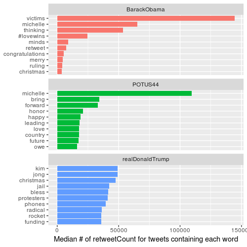
Words that are most likely to be in a retweet
Use the same code as above, but replace retweetCount with favoriteCount:
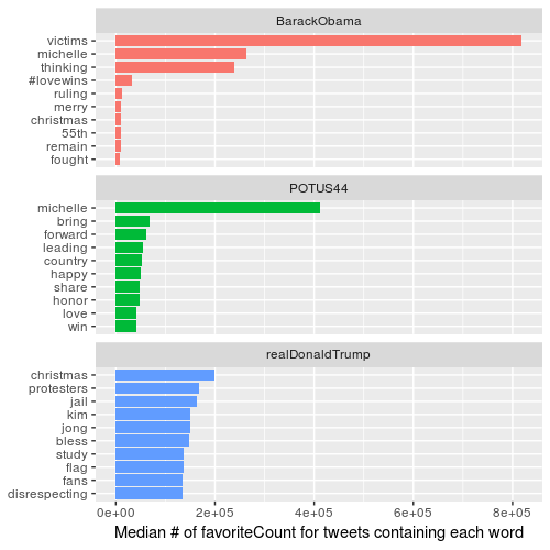
Words that are most likely to be in a favorite
There’s a interesting change of pattern between Trump’s retweets and favorites. It seems there are some tweets people would rather retweet than favorite, and vice versa.
The End
Thanks for reading! Please support the author of the book (I have no affiliation with them) if you like the tidytext package and the book.
You can find the source code of this post on RPubs: RPubs - Trump & Obama Tweets Analysis.