
Overview
Kaggle recently hosted a competition (Instant Gratification) to test their new “synchronous Kernel-only competition” format. It features a synthetic dataset, and the best way to achieve high score on this dataset is to reverse-engineer the dataset creation algorithm.
I did not really spend time into this competition, but after the competition was over I went back checked the discussion forum for solutions and insights shared, and found it actually quite interesting. There are quite a few of lessons to be learned about how to create or deal with synthetic data.
The Revelation
This is the function call that we want to reverse-engineer from data:
X,y = make_classification(
    n_samples=NUM_SAMPLES,
    n_features=NUM_FEATURES,
    n_informative=random.randint(33,47),
    n_redundant=0,
    n_repeated=0,
    n_classes=2,
    n_clusters_per_class=3,
    weights=None,
    flip_y=0.05,
    class_sep=1.0,
    hypercube=True,
    shift=0.0,
    scale=1.0,
    shuffle=True,
    random_state=random_seed)
The competition dataset consists of 512 sub-dataset created by the above function call, and a “magic” discrete feature is attached so we can perfectly tell them apart.
Cracking Each Parameter
- n_informative: Can be found by removing uninformative features (detail described later).
- n_redundant: Linear combination of informative features. Keeping them should not affect model accuracy. But they’ll make infering other parameters more complicated. The existence of such features can be detected using multicollinearity tests, but to exactly identify them is much harder. If
n_clusters_per_classis low andn_samplesis large enough, we might have some good guesses by looking at empirical feature means grouped by targets - n_repeated: Given the amount of features, brute force search alone can do the trick.
- n_clusters_per_class: This is the most tricky part. Luckily the actual number is low enough so we can crack it using data visualization (details described later).
- flip_y: Nothing really can be done with this one. We can only empirically find that about 2.5% data points cannot be correctly lassified even after we cracked all other parameters. With only two classes, that means 5% of the target labels were randomly exchanged.
- class_sep: Found by the visualization used to find
n_clusters_per_class. - hypercube: Found by the visualization used to find
n_clusters_per_class. Things will be much harder ifhypercubeis false. - shift: If constant, can be found by visualizing the empirical feature means. Would be much complicated if it’s random.
- scale: Same as
shift.
As you can see, the competition can make a lot harder by changing some of the parameters. Many competitors were able to create perfect classifier by the end of the competition, and their ranking are determined by the randomness introduced by flip_y parameter.
Uninformative Features
As we’ve just mentioned, this competition used make_classification from scikit-learn to create synthetic data. According to the documentation:
The remaining (uninformative) features are filled with random noise.
It turns out that the random noise is Guassian distributed with zero mean and unit variance. The unit cariance is in stark contrast to the variance of other informative features, making them very easy to identify:
px.histogram(
   pd.DataFrame(dict(stdev=subset_train[cols].std(axis=0).values)),
   x="stdev", nbins=30, width=768, height=384, title="Feature Stdandard Deviation",
   template="plotly_white"
)
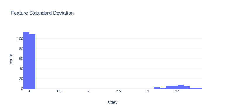
Distribution of standard deviation of feature values.
One potential alternative way to create uninformative features is to take some informative features and randomly shuffle them.
Another interesting observation is that the variances of informative features are not constant. The plot below was created by running:
X_dummy, y_dummy = make_classification(
    n_samples=1024, n_features=1, n_informative=1, n_redundant=0, n_repeated=0,
    n_classes=2, n_clusters_per_class=1, flip_y=0, class_sep=1.,
    hypercube=True, scale=1, shift=0.0,
)
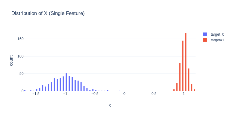
Two clusters have different variances.
And the variance increases as the number of informative features increases (otherwise adding more informative features will make the problem easier):
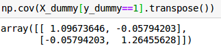
Covariance matrix with 2 features.
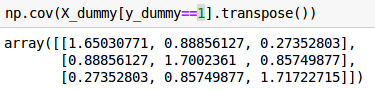
Covariance matrix with 3 features.
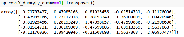
Covariance matrix with 5 features.
The Number of Clusters per Class
Deciphering the n_clusters_per_class is the critical step to get perfect classifiers. The most popular model in this competition — QDA(Quadratic Discriminant Analysis) — only fits the case where n_clusters_per_class = 1, because the underlying assumption of QDA is that data of each class follows a single multivariate Guassian distrbution. Having more than one (Gaussian) cluster per class breaks that assumption.
Solution #1: EDA / Data Visualization
I failed to think of the solution which Chris Deotte described in this notebook. But it only works when n_clusters_per_class is small and n_samples is sufficiently large.
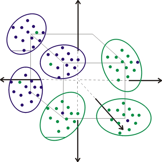
The solution is to plot histogram of the feature means grouped by targets across all 512 sub-datasets, and compare the plot with the plots from simulated runs. Because hypercube=True, shift=0, scale=1., and class_sep=1, the cluster means in each dimension can only located at either 1 or -1. The histogram should thus describes a shifted binomial distribution with some random noises. For example, if n_clusters_per_class=2, there can only be three possible feature means (-1-1, -1+1, 1+-1, 1+1) / 2:
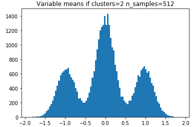
Population means: -1, 0, 1
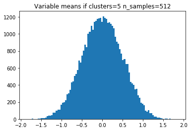
The competition dataset actually looks like this:
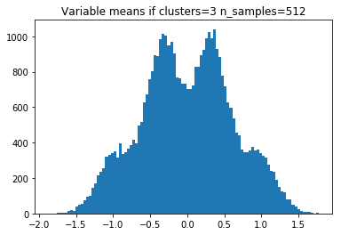
Population means: -1, -0.33, 0.33, 1
And from this, we’ve learned that there are three clusters per class.
Cases where It Doesn’t Work
We cannot do it in a unsupervised manner, that is, calculate feature means without grouping by target. By doing that each feature mean would count samples from 6 clusters instead of 3. And a binomial distribution with n=6 and p-0.5 already looks a lot similar to a normal distribution:
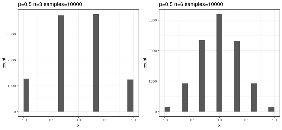
X axes have been shifted and scaled
Since we’re dealing with sample (feature) means, the random noises will make it very hard to tell if the number of clusters is 5, 6, 7, 8, or more.
Therefore, it’s critical that we group the features values by target to make the number of clusters accounted smaller. Although we have 2.5% of rows with flipped target, the percentage not big enough to interfere the decision.
Another important factor is the number of samples. Without enough samples, the variance of sample means will be too large and the histograms will become indistinguishable.
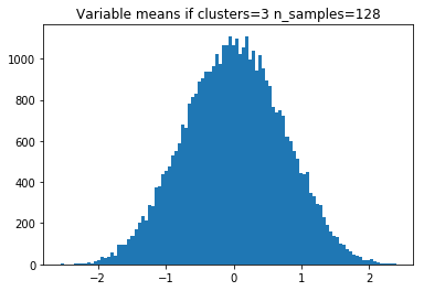
128 samples per feature
To avoid insufficient number of samples, we can pseudo-labels(use a model to generate prediction and treat the prediction as true label) test dataset and include them in our sample mean calculation.
Solution #2: Directly Fitting Gaussian Mixture Model
This idea comes from this Cross Validated thread. We want to determine the number of underlying clusters our Guassian Mixture model should use. We can try several possible options and evaluate the log-likelihood or BIC(Bayesian information criterion) of the fitted models. The one with the largest log-likelihood or lowest BIC is the most likely number of clusters:
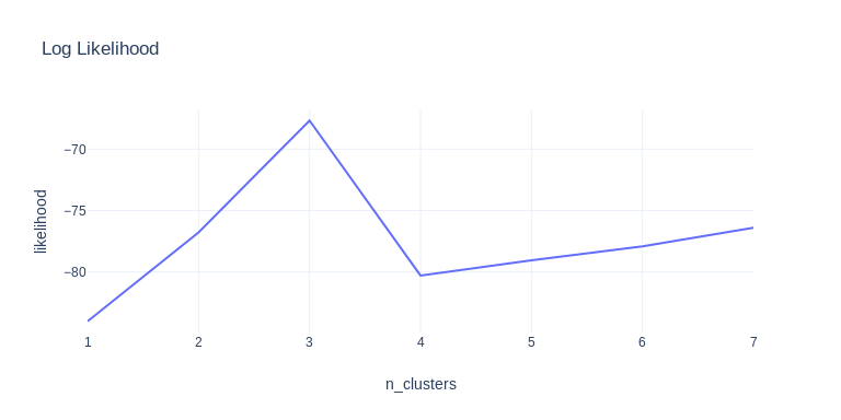
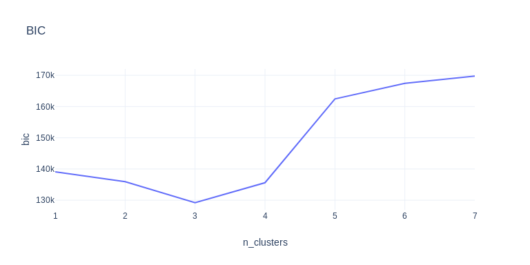
This solution can handle larger n_clusters_per_class given enough samples. The number of samples is very important because the model need to estimate the covariance matrix of each cluster.
If we only use train dataset, which have 512 samples per sub-dataset in average and around 40 informative features. That leaves around 85 samples to estimate the 40x40 covariance matrix, which can be quite unstable.
For this dataset, if we fit a Gaussian mixture model on train dataset only unsupervised, the evaluation method described above wouldn’t be able to tell us the correct number of clusters, and the validation trick described in the thread won’t work (using the test dataset as validation). But if we include the test data when fitting the model, the correct number of cluster will come out most of the time. So you just need to run the evaluation a couple dozen times and pick the most common answer. But of course, the best way to do it is utilizing the target labels as described in the previous section, and preferably try to fix some obviously flipped samples.
Summing up
Once we figured out that n_clusters_per_class=3, we can fit the dataset almost perfectly using a Gaussian Mixture Model. The final missing piece is find some way to fix some of the flipped labels so the model would be more stable. Setting some hard threshold seems to suffice for this dataset as observed in some top solutions.
This is a really interesting competition. It challenges my understanding of some key concepts (very rusty in some cases, as it turned out). There are still some more stuffs I’d like to experiment on but did not given the time constraint (possible future updates?).
Making use of synthetic data IMO is a key skill of data scientist since real data can be very expensive to obtain. You’d want to make sure your system is ready for real data before you spend resources collecting more of them. Knowing how to make the synthetic data hard enough and/or similar to real data enough can save you and your company a lot of time and trouble.