
Introduction
Jigsaw toxic comment classification challenge features a multi-label text classification problem with a highly imbalanced dataset. The test set used originally was revealed to be already public on the Internet, so a new dataset was released mid-competition, and the evaluation metric was changed from Log Loss to AUC.
I tried a few ideas after building up my PyTorch pipeline but did not find any innovative approach that looks promising. Text normalization is the only strategy I had found to give solid improvements, but it is very time consuming. The final result (105th place/about top 3%) was quite fitting IMO given the time I spent on this competition(not a lot).
(There were some heated discussion around the topic of some top-ranking teams with Kaggle grand masters getting disqualified after the competition ended.)
Public kernel blends performed well in this competition (i.e. did not over-fit the public leaderboard too much). I expected it to overfit, but still selected one final submission that used the best public blend of blends to play it safe. Fortunately it paid off and gave me a 0.0001 boost in AUC on private leaderboard:
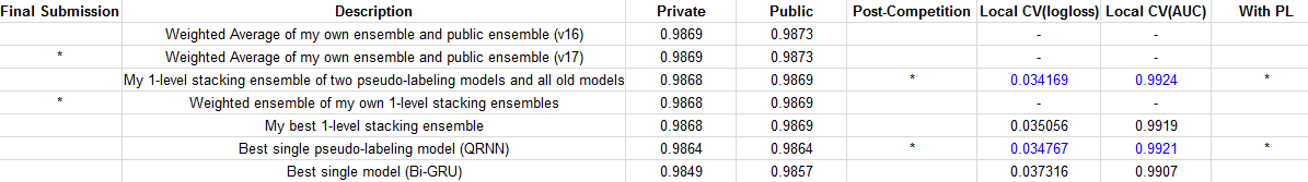
Table 1: Selected submissions in descending order of private scores
In this post, I’ll review some of the techniques used and shared by top competitors. I do not have enough time to test every one of them myself. Part 2 of this series will be implementing a top 5 solution by my own, if I ever find time to do it.
List of Techniques
I tired to attribute techniques to all appropriate sources, but I’m sure I’ve missed some sources here and there. Not all techniques are covered because of the vast amount of contents shared by generous Kagglers. I might come back and edit this list in the near future.
- Translation as Augmentation (test time and train time) [1][2][13]
- Pseudo-labelling [1]
- Text normalization [3][4]
- Multi-level stacking — 4 levels [3]; 2 levels [11]; 1level stacking + 1 level weighted averaging [12]
- Non-English embeddings [2]
- Diverse pre-trained embeddings — Train multiple model separately on different embeddings
- Combine several pre-trained embeddings — concatenate after a RNN layer [3]; Concatenate at embedding level [5]; Variant of Reinforced Mnemonic Reader [7]
- When truncating texts, retain both head and tail of the texts [1]
- K-max pooling[6]
- Multiple-level of stacking [3]
- Deepmoji-style attention model [3]
- (NN) Additional row-level features:“Unique words rate” and “Rate of all-caps words”[4]
- (NN) Additional word-level feature(s): If a word contains only capital letters [4]
- (GBM) Engineered features other than tf-idf [12]
- BytePair Encoding [5][8]
- R-net [7]
- CapsuleNet [11]
- Label aware attention layer [7]
- (20180413 Update) leaky information — small overlaps of IPs between training and testing dataset. One overlapping username. [14]
Pseudo-labelling and Head-Tail Truncating
I’ve already tried these two techniques and trained a couple of models for each.
Head-tail truncating (keeping 250 tokens at head, 50 tokens at tail) helped only a bit for bi-GRU, but not for QRNN. It basically had no effect on my final ensemble.
For pseudo-labelling(PL), I used the test-set predictions from my best ensemble as suggested in [1], and they improved the final ensemble a little (see table 1). I’d assume that adding more model trained with PL will further boost the final AUC. However, the problem of this approach is the leakage it produces. The ensemble model had seen the the all the validation data, and that information leaked into its test set predictions. So the local CV will be distorted and not comparable to those trained without PL. Nonetheless, this technique does create the best single model, so it’ll be quite useful for production deployment.
I think the more conservative way of doing PL is to repeat the train-predict-train(with PL) process, so the model is trained twice for every fold. But that’ll definitely takes more time.
References:
- The 1st place solution overview by Chun Ming Lee from team Toxic Crusaders
- The 2nd place solution overview by neongen from team neongen & Computer says no
- The 3rd place solution overview by Bojan Tunguz from team Adversarial Autoencoder
- About my 0.9872 single model by Alexander Burmistrov from team Adversarial Autoencoder
- The 5th place brief solution by Μαριος Μιχαηλιδης KazAnova from team TPMPM
- Congrats (from ghost 11th team) by CPMP
- The 12th place single model solution share by BackFactoryVillage from team Knights of the Round Table
- The 15th solution summary: Byte Pair Encoding by Mohsin hasan from team Zehar 2.0
- The 25th Place Notes (0.9872 public; 0.9873 private) by James Trotman (solo)
- The 27th place solution overview by Justin Yang from team Sotoxic
- The 33rd Place Solution Using Embedding Imputation (0.9872 private, 0.9876 public) by Matt Motoki (solo)
- The 34th, Lots of FE and Poor Understanding of NNs [CODE INCLUDED] by Peter Hurford from team Root Nice Square Error :)
- A simple technique for extending dataset by Pavel Ostyakov
- The 184th place write-up: code , solution and notes(without blend) by Eric Chan