
Motivation
I was reading this paper titled “Character-Level Language Modeling with Deeper Self-Attention” by Al-Rfou et al., which describes some ways to use Transformer self-attention models to solve the language modeling problem. One big problem of Transformer models in this setting is that they cannot pass information from one batch to the next, so they have to make predictions based on limited contexts.
It becomes a problem when we have to compare the results with “traditional” RNN-based models, and what Al-Rfou et al. proposed is to use only the outputs at the last position in the sequence from the Transformers when evaluating. If we ignore the first batch, a sequence of length N will require N batches to predict for Transformers, and only (N / M) batches for RNN models (M being the sequence length of a batch).
As I read the paper, I’d found that I was not really sure about some implementation details of RNN-based language models. It really bugged me, so I went back to the official PyTorch example and figured it out. The following sections are the notes I took during the process.
Theoretical Background
We’re not going to cover this in this post. But here are some resources for you if you’re interested:
-
[Video] Lecture 8: Recurrent Neural Networks and Language Models — Taught by Richard Socher, who is an excellent teacher. Highly recommended.
-
Gentle Introduction to Statistical Language Modeling and Neural Language Models
Basically a language model tries to predict the next token given the previous tokens, which is to estimate the conditional probability:
Source Code
I forked the pytorch/examples Github repo, made some tiny changes, and added two notebooks. Here’s the link:
Dataset Preparation
This example comes with a copy of wikitext2 dataset. The texts have already been tokenized to word level, and split into train, validation, test sets.
No processing is needed other than replacing newlines with <eos> tokens.
Line 30–38 construct the dictionary (word to index mapping) with a full scan. Then line 41–50 use that dictionary to convert the words into numbers, and store the numbers in a single PyTorch tensor. For example, the sentence “This is me using PyTorch.” can become LongTensor([0, 1, 3, 5, 4, 6]).
In Wikitext2, there is an empty line before and after section titles. I don’t think we need to keep those empty lines because section titles are already clearly identifiable to machines by the consecutive = tokens, so I add line 33–34 and line 45–46 to skip them. It’ll hurt the perplexity slightly because previously we can easily predict another <eos> right after an <eos> at the end of a section title.
I also added a strip call at line 35 and 47 just to make sure. And it turned out wikitext2 is clean enough. The number of tokens collected remains the same.
After initialization, a Corpus object will contain one dictionary object, and three 1-dimensional LongTensor objects.
Batchify
This is best explained in examples. Suppose we want a batch size of 4, and we have a 1-dimensional tensor containing 38 numbers in ascending order — [1, 2, …, 38]. (It is extremely simplified just to make the example more readable.)
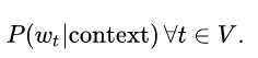
In line 3 we have nbatch = 38 // 4 = 9. In line 5 we have nbatch * bsz = 36, and therefore discard the last two numbers (37 and 38). In line 7 we transform the 36 numbers into a 9x4 2-dimensional tensor. For readability’s sake we’ll visualize it as a 4x9 tensor:
The resulting 4 x 9 tensor
Model
This example uses very basic GRU/LSTM/RNNmodels you can learn from any decent tutorials on the topic of recurrent neural networks. We’re not going to cover it in detail. You can read the source code here:
ceshine/examples/word_language_model/model.py
Training: Iterating Through Batches
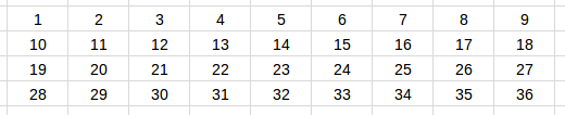
The parameter bptt (backpropagation through time) is the longest time step backward we want the gradient to backpropagate to, which will be the sequence length of the batch. Continuing our example, suppose we want a bptt of 3, each batch will contain one 3x4 input tensor and one 3x4 target tensor, except for the last batch.
Let’s start from the first batch (again, we transpose the tensor for easier visualization):
The first batch: input tensor (4 x 3))
The first batch: target tensor (4 x 3)
Hidden states are initialized as zeros with shape (self.nlayers, bsz, self.nhid). Note that each example(row) in a batch gets its own hidden states.
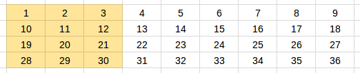
After we’re done training the first batch (feed-forward and backpropagate), we repackage the hidden states (detach them from the graph so there will be not backpropagation beyond them), and move on to the next batch:
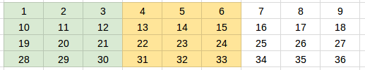
Yellow — The second batch: input tensor (4 x 3). Green — inputs that have been seen by the model.
The second batch: target tensor (4 x 3)
Because we reuse the hidden states, the recurrent unit that are fed the sequence [4, 5, 6] has already seen sequence [1, 2, 3]. Theoretically it’ll be able to make better predictions based on this context. In this case, the model can be more confident in the prediction that this is a increasing arithmetic sequence.
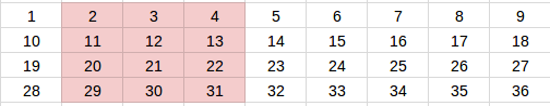
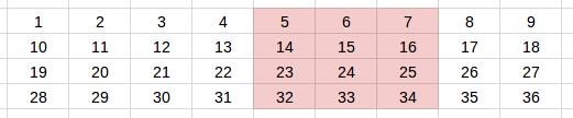
We then train this batch and repackage the hidden states just like the first batch. And here comes the tricky part — the third and final batch.
In line 9 we have seq_len = min(args.bptt, len(source) — 1 — i). After dealing with the second batch, i would be 6, and len(source) — 1 — iwould be 2, less than our bptt(3). This is because we need to have a proper target tensor for the supervised model.
Yellow — The third batch: input tensor (4 x 2). Green — inputs that have been seen by the model.
The third batch: target tensor (4 x 2)
That’s it! We’ve completed an epoch. Note that we are not able to shuffle the batches as we usually do in other situations, because the information is passed between batches. This will make input and target tensors in each epoch exactly the same. To alleviate this problem, we can try to randomize the bptt parameter. An example implementation is in the Github salesforce/awd-lstm-lm repo. Fastai library also use a similar algorithm.
Evaluation
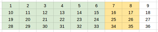
Here’s the part most confused me. The batch size of the evaluation phase clearly affects the evaluation result. Here’s an example to demonstrate this. Suppose the evaluation set consists of 5 series with the same length and the same values [1, 2, …, 8]. One of the better scenarios is using a batch size of 5:
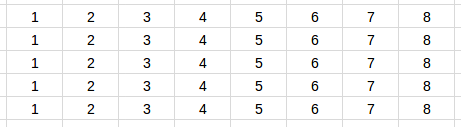
Batchify scheme as a 5 x 8 tensor
Each recurrent unit will be able to get as much context information about a series as possible.
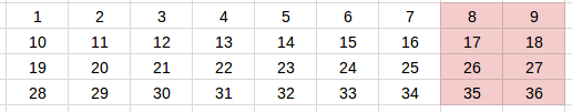
Now consider a different batch size (6):
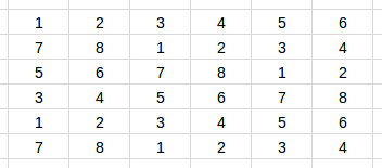
A less ideal batchify scheme as a 6 x 6 tensor
Not only we discarded 4 entries in the evaluation set, we also distributed 5 series into 6 rows. It makes things harder for the model. For example, if the model has learned that if it has already seen [3, 4, 5, 6, 7], then the next number will highly likely to be 8. But in the second row the model can only see a 7, and is not able to use the previously learned pattern.
The 6 x 6 batchify scheme will very likely have a higher perplexity (lower is better) than the 5 x 8 one.
I think the safest batchify scheme is not batchify at all. Just use a batch size of 1. It’ll require much more time to predict, but is the most robust and consistent way. This is what salesforce/awd-lstm-lm did (test_batch_size = 1), but unfortunately not the PyTorch example.
However, if the dataset is large enough relative to the batch size, the effect of this problem will likely be negligible, as only a small fraction of sentences or documents are being cut into two pieces.
Training and Evaluating on Google Colaboratory
Thanks to Google Colab, we can run the entire training and evaluation process for free on the Internet. The training time for the small model in the example is about 4 hours.
I’ve provided bash commands and training log in the notebook below:
(The perplexity given in the README seems to be from the PTB dataset, and is lower than the one we get from the wikitext2 dataset.)
The maximum lifetime of a Google Colab VM is 12 hours. You’ll want to download the trained model to your computer. I couldn’t get this to work (the connection is reset after a while) and have to resort to using Cloud Storage:
from google.colab import files
files.download('model.pt')
Maybe you’ll have better luck. Try replicate the example or train a bigger model yourself. Remember to enable GPU in Runtime / Change Runtime Type / Hardware Accelerator.
I’ve also provided a notebook that loads and evaluate the mode:
It reruns the evaluation process for the test dataset, to make sure we have loaded the correct model. It also contains code that displays predictions for humans to examine by eye, and code that generates texts based on the given contexts.
One other way to evaluate language models is to calculate the probabilities of sentences. Sentences that do not make sense should have much lower probabilities than those that make sense. I haven’t implemented this yet.
Fin
Thanks for reading! Please feel free to leave comments and give this post some claps if you find it useful.