Playing with rstudio/gt R Package

Tables can be an effective way of communicating data. Though not as powerful in telling stories as charts, by cramming a lot of numbers into a limited space, tables can provide readers with accurate and potentially useful information which readers can interpret in their own ways.

I’ve come across this new R package gt (Easily generate information-rich, publication-quality tables from R) and decided to give it a try.

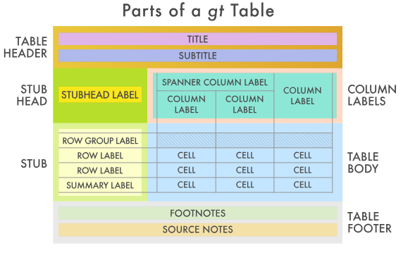
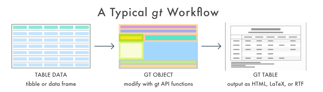
With the gt package, anyone can make wonderful-looking tables using the R programming language. The gt philosophy: we can construct a wide variety of useful tables with a cohesive set of table parts. These include the table header, the stub, the stub head, the column labels, the table body, and the table footer.

Admittedly, the tables in my attempt might not be the optimal way of presentation. They serve as a demonstration of what gt can do, and maybe also helpful enough for analyst in constructing their stories about this dataset (The Movies Dataset on Kaggle).

(kaggle.com) The Movies Dataset: Metadata on over 45,000 movies. 26 million ratings from over 270,000 users.

Cheat Sheet

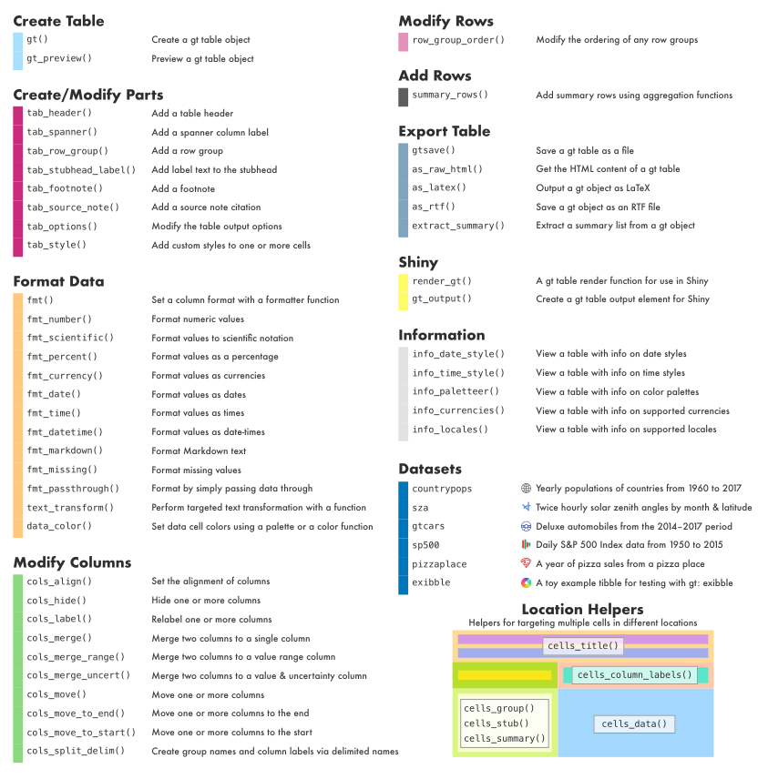
Source Code (Rendered RMarkdown)

You can find the full source code here:

(rpubs.com) RPubs — Movie Genre Overlappings, Ratings by Genre and Year

Or this Github Repo:

ceshine/movies_dataset_eda

The Github repo contains a Dockerfile and packrat configurations. Please refer to this previous post for more information:

More Portable, Reproducible R Development Environment

(Unfortunately, I couldn’t installrstudio/gt in Kaggle Kernel. Otherwise, it would be a great place to host the rendered document.)

Genre Statistics

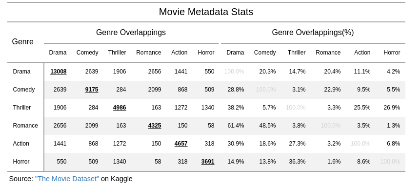
How to read the table: For example, Drama (the first row) has 13008 movies (the first column), and 2639 of them are also under Comedy, which is 20.3% of the 13008 movies.

The data in each section is symmetric, so I wasted almost half the data cells. A more clever way is to use one of the upper or lower triangles for raw counts, and the other for percentages.

Interesting features:

Making texts in the diagonal cells in the “Genre Overlappings” section bold and add underlines:

tab_style(
style = cells_styles(
text_decorate = "underline",
text_weight = "bold"),
locations = list(
cells_data(columns=c(1), rows=c(1)),
cells_data(columns=c(2), rows=c(2)),
cells_data(columns=c(3), rows=c(3)),
cells_data(columns=c(4), rows=c(4)),
cells_data(columns=c(5), rows=c(5)),
cells_data(columns=c(6), rows=c(6))
))

Displaying the numbers in the “Genre Overlappings(%)” section in percentage format:

fmt_percent(
columns = vars(Drama.ratio, Comedy.ratio, Thriller.ratio,
Romance.ratio, Action.ratio, Horror.ratio),
decimals = 1,
drop_trailing_zeros = F
)

Movie Ratings by Genre

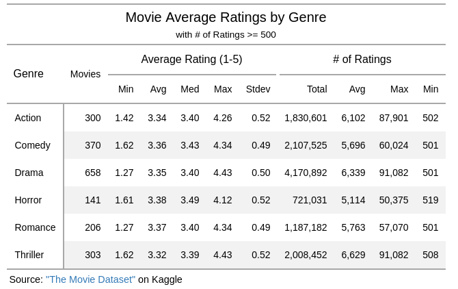
Surprisingly, the distributions of ratings are quite similar across all genres. Maybe MovieLens has done some normalization on the ratings?

Movie Ratings by Genre and Year(Decade)

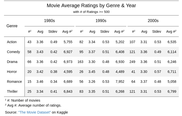
It appears the variances of ratings in the 1980s are lower than in the 1990s and the 2000s. (A boxplot or scatterplot might actually be more appropriate here.)

Adding footnotes:

tab_footnote(
footnote = "#: Number of movies",
cells_column_labels(columns = c(1, 5, 9))
) %>%
tab_footnote(
footnote = "Avg #: Average number of ratings.",
cells_column_labels(columns = c(4, 8, 12))
)

I did not find any way to change the text style of the footnotes, though.

Conclusion

The rstudio/gt package is still in early development stage and hasn’t been released to CRAN yet. However, it already shows great promises and can be extremely helpful in creating beautiful tables in your reports and documents.

There are still plenty of the rstudio/gt features I did not cover in this post (e.g., row groups). I’m sure more awesome example usage of this package will soon emerge from the community. Stay tuned!