
We’ve discussed what quantile regression is and how does it work in Part 1. In this Part 2 we’re going to explore how to train quantile regression models in deep learning models and gradient boosting trees.
Source Code
The source code to this post is provided in this repository: ceshine/quantile-regression-tensorflow. It is a fork of strongio/quantile-regression-tensorflow, with following modifcations:
-
Use the example dataset from the scikit-learn example.
-
The TensorFlow implementation is mostly the same as in strongio/quantile-regression-tensorflow.
-
Add an example of LightGBM model using “quantile” objective (and a scikit-learn GBM example for comparison) based on this Github issue.
-
Add a Pytorch implementation.
-
Provide a Dockerfile to reproduce the environment and results.
-
In addition to .ipynb notebook files, provide a .py copy for command line reading.
Tensorflow
The most important piece of the puzzle is the loss function, as introduced in Part 1:
Loss Function of Quantile Regression (Source)
The tricky part is how to deal with the indicator function. Using if-else statement on each example would be very inefficient. The smarter way to do it is to calculate both y _ τ and y _ (τ-1) and take element-wise maximums (this pair will always have one positive and one negative number except when y=0. τ is in (0, 1) range.).
The following implementation is directly copied from strongio/quantile-regression-tensorflow by @jacobzweig:
error = tf.subtract(self.y, output)
loss = tf.reduce_mean(tf.maximum(q*error, (q-1)*error), axis=-1)
If using this implementation, you’ll have to calculate losses for each desired quantile *τ *separately. But I think since we usually only want to predict only 2 to 3 quantiles, the need to optimize this is insubstantial.
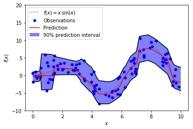
The rest is just regular Tensorflow neural network building. You can use whatever structure you want. We give an example here fitting the example dataset from scikit-learn:
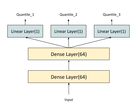
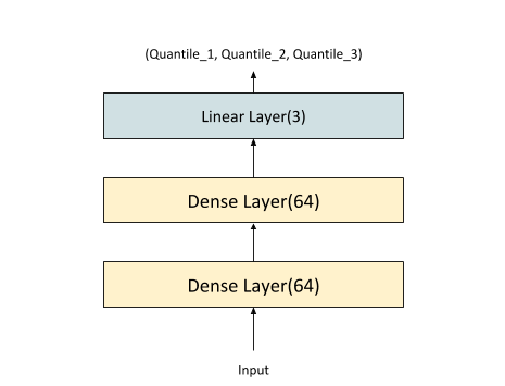
The final layers can be made even simpler by using one big linear layer at the top. The underlying calculations are exactly the same, but the latter implements it in a big weight matrix (and a bias vector). The PyTorch implementation we’re going to see later provides an implementation of this approach:
The fitted model would look like this:
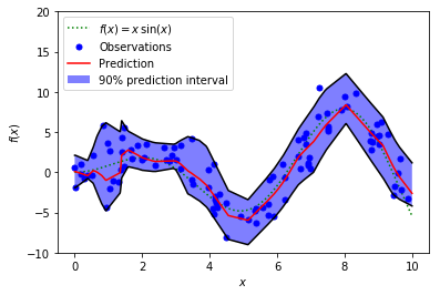
Tensorflow Implementation
PyTorch
The loss function is implemented as a class:
class QuantileLoss(nn.Module):
    def __init__(self, quantiles):
        super().__init__()
        self.quantiles = quantiles

    def forward(self, preds, target):
        assert not target.requires_grad
        assert preds.size(0) == target.size(0)
        losses = []
        for i, q in enumerate(self.quantiles):
            errors = target - preds[:, i]
            losses.append(
                torch.max(
                   (q-1) * errors,
                   q * errors
            ).unsqueeze(1))
        loss = torch.mean(
            torch.sum(torch.cat(losses, dim=1), dim=1))
        return loss
20180718 Edit: Fixed a bug inside forword() method. Should have used self.quantiles instead of quantiles. Lesson learned: avoiding reusing variable names in Jupyter notebooks, which usually are full of global variables.
It expects the predictions to come in one tensor of shape (N, Q). The final torch.sum and torch.mean reduction follows the Tensorflow implementation. You can also choose use different weights for different quantiles, but I’m not very sure how it’ll affect the result.
PyTorch Implementation
Batch Normalization
One interesting I noticed is that adding batch normalization makes the PyTorch model severely under-fit, but the Tensorflow model seems to fare better. Maybe it’s the very small size of batches(10) and the small training dataset (100 examples) that’s causing problems. The final version has batch normalization from both model removed. Training models on a larger real-world dataset, which has yet to be done, should help me figuring it out.
Monte Carlo dropout
I’ve covered Monte Carlo dropout previously in this post: [Learning Note] Dropout in Recurrent Networks — Part 1: Theoretical Foundations.
In short, it performs dropout in test/prediction time to approximate sampling from the posterior distribution. The we can find the credible interval for a quantile. We show the credible interval of the median below:
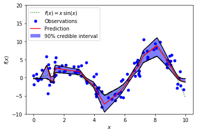
Tensorflow MC Dropout for the Median
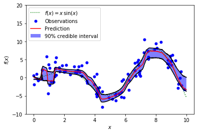
PyTorch MC Dropout for the Median
As we can see, the credible interval is much narrower than the prediction interval (check Part 1 if you’re not sure what they mean). These two can be quite confusing, as stated in the following discussion thread (Check Ian Osband’s comment):
In Osband’s comment, “the posterior distribution for an outcome” is used to construct the prediction interval, and “posterior distribution for what you think is the mean of an outcome” is used to construct the credible interval. He also gave an clever example to demonstrate their differences:
A fair coin, that you know is a fair coin. You can be 100% sure that the expected outcome is 0.5. This is the posterior distribution for the mean — a dirac at 0.5. On the other hand, for any single flip the distribution of outcomes is 50% at 0 and 50% at 1. The two distributions are completely distinct.
I think you’ll have to find some way to sample from the posterior distribution of the error term to create prediction intervals with MC dropout. Not sure how to do it yet. Maybe we can estimate the distribution by collecting the errors when sampling the target (I need to do more research here).
LightGBM
For tree models, it’s not possible to predict more than one value per model. Therefore what we do here is essentially training Q independent models which predict one quantile.
Scikit-learn is the baseline here. What you need to do is pass loss=’quantile’ and alpha=ALPHA, whereALPHA((0,1) range) is the quantile we want to predict:
Scikit-Learn GradientBoostingRegressor
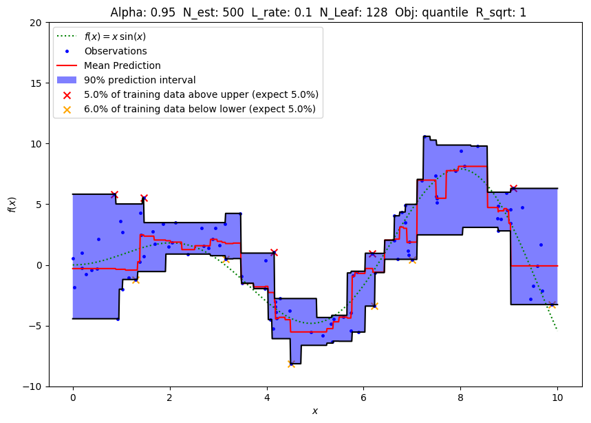
LightGBM has the exact same parameter for quantile regression (check the full list here). When using the scikit-learn API, the call would be something similar to:
clfl = lgb.LGBMRegressor(
    objective = '**quantile**',
    **alpha** = 1 - ALPHA,
    num_leaves = NUM_LEAVES,
    learning_rate = LEARNING_RATE,
    n_estimators = N_ESTIMATORS,
    **min_data_in_leaf**=5,
    reg_sqrt = REG_SQRT,
    max_depth = MAX_DEPTH)
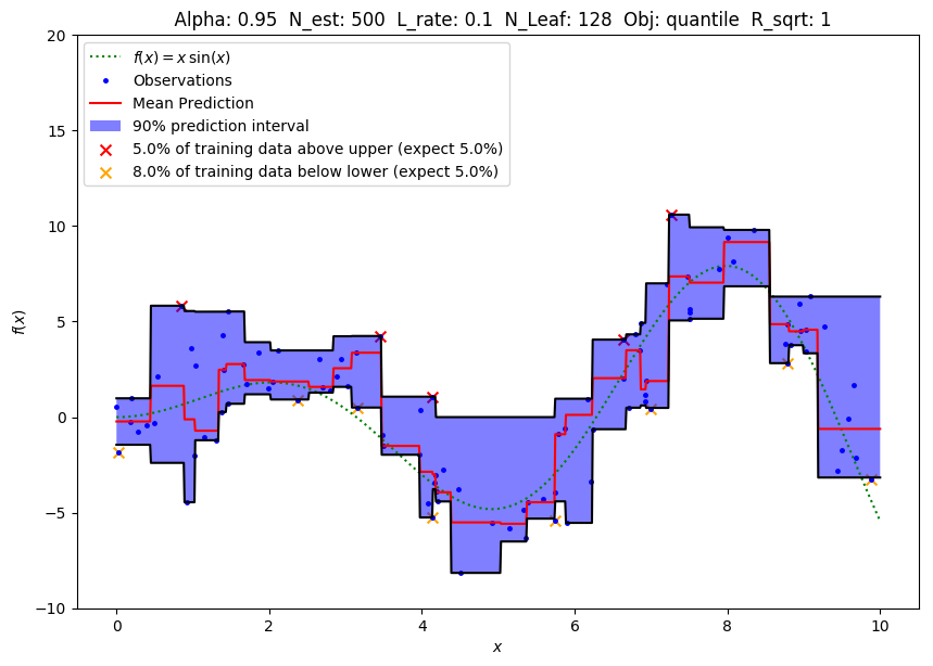
LightGBM LGBMRegressor
One special parameter to tune for LightGBM — min_data_in_leaf. It defaults to 20, which is too large for this dataset (100 examples) and will cause under-fit. Tune it down to get narrower prediction intervals.
Not much to say here. The gradients of the loss function are handled inside the library. We only need to pass the correct parameter. However, unlike neural networks, we cannot easily get confidence interval nor credible interval from tree models.
The End
Thank you for reading this far! Please consider give this post some claps to show your support. It’ll be much appreciated.