
This post summarizes the findings and suggestions from the paper “Please Stop Permuting Features ‒ An Explanation and Alternatives” by Giles Hooker and Lucas Mentch.
(Note: Permutation importance is covered in one of my previous posts: Feature Importance Measures for Tree Models — Part I.)
TL;DR
Permutation importance (permuting features without retraining) is biased toward features that are correlated. Avoid using it, and use one of the following alternatives:
- Conditional variable importance: permute or generate the feature data from the distribution conditioned on other features
$x^{c,j}_{ij} \sim x_{ij} | x_{i, -j}$, then calculate the difference in loss using the same model (no retrain). - Dropped variable importance (leave-out-covariates (LOCO)): drop the target feature and retrain the model. Calculate the difference in loss between the two models.
- Permute-and-relearn importance: permute the feature data and retrain the model. Calculate the difference in loss between the two models.
- Conditional-and-relearn importance: permute or generate the feature data from the distribution as in conditional variable importance, but retrain the model and compare the difference in loss.
(Another alternative is the SHAP values, which is covered in this post of mine: [Notes] SHAP Values).
We don’t discuss partial dependence plots (PDPs) and individual conditional expectation plots (ICE) in this post because there is no good alternative available (for now). In general, we should not use them with permutation methods.
Introduction
Permutation importance (simply called “variable importance” in this paper) is defined by Breiman (2001) as:
where $X^{\pi,j}_{i}$ is a matrix achieved by randomly permuting the j th column of X.
This feature importance measure is computationally cheap, applies to the $f(x)$ derived from any learning method, has no tuning parameters, and statistically very stable. Therefore, they are frequently adopted and advocated for the general public.
However, this permute-and-predict (PaP) structure has serious flaws, especially when significant correlations exist between features. It has been demonstrated in multiple studies (Strobl et a. (2007); Archer and Kimes (2008); Nicodemus et al. (2010)).
This paper provides an intuitive rationale for the flaws. It argues that when two features are highly correlated, there will be a lot of areas on the hyperplane that don’t have training examples. When one of the features got permuted, the model will be forced to extrapolate. As the quality of extrapolation is usually very low in more complicated models, the loss will deteriorate sharply, making the permutation importance measure putting more weight on this feature.
A Simple Simulation Example
This paper argues that permutation-based diagnostic tools are misleading when both of these conditions are met:
- A flexible learning method is used.
- The data has correlated features.
A simple artificial dataset demonstrated the influence of these two conditions for us. The dataset is generated from this linear model:
where $\epsilon_{i} \sim N(0, 0.1^2)$. Each of the features is marginally distributed as uniform on [0, 1]. They are generated independently except for the first two ($x_{1}$, $x_{2}$).
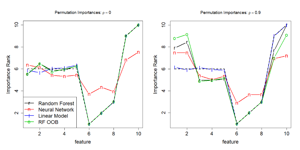
Figure 1 from the paper
From the simulation result, we can see that all the models agree on the same feature importance ranking when all features are independent (condition 2) and that neural network and random forest rank the correlated features higher while a linear model does not (condition 1).
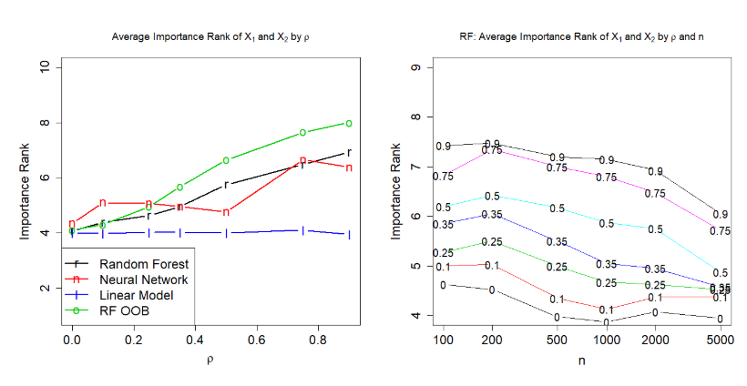
Figure 2 (partial) from the paper
The increase in the correlation coefficient exacerbates the problem, as does the decrease in training examples.
Extrapolation and Explanations
If we simplify the linear model behind the artificial dataset to $y = x_1 + \epsilon$ and plot the contours of the learned random forest, we get:
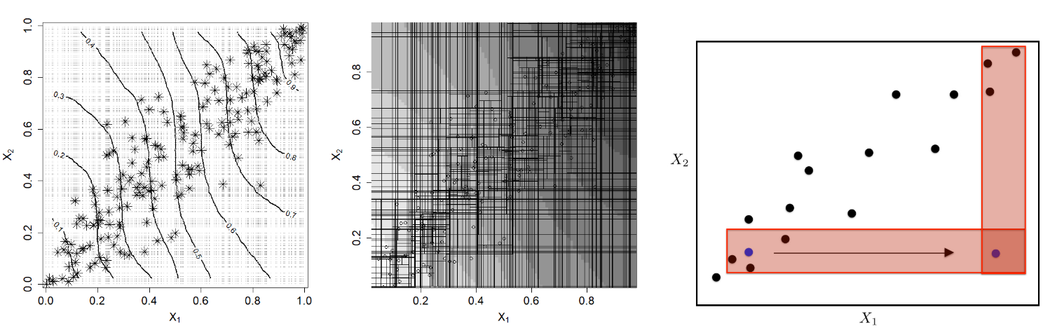
Figure 4 from the paper
We know that the true contours should be vertical lines, and we can see that the random forest only approximate these contours within the convex hull of the data. When one of the features get permuted, the data points will usually land on the bottom right or upper left of the plot, where the contour is highly distorted.
Because of how tree model works, the predicted value of x is determined by the “potential nearest neighbours” in the training examples (the plot on the right in Figure 4). The potential nearest neighbours judged from the two features are highly incongruous, thereby heavily disrupt the predictions, and make the PaP structure biased towards these two features.
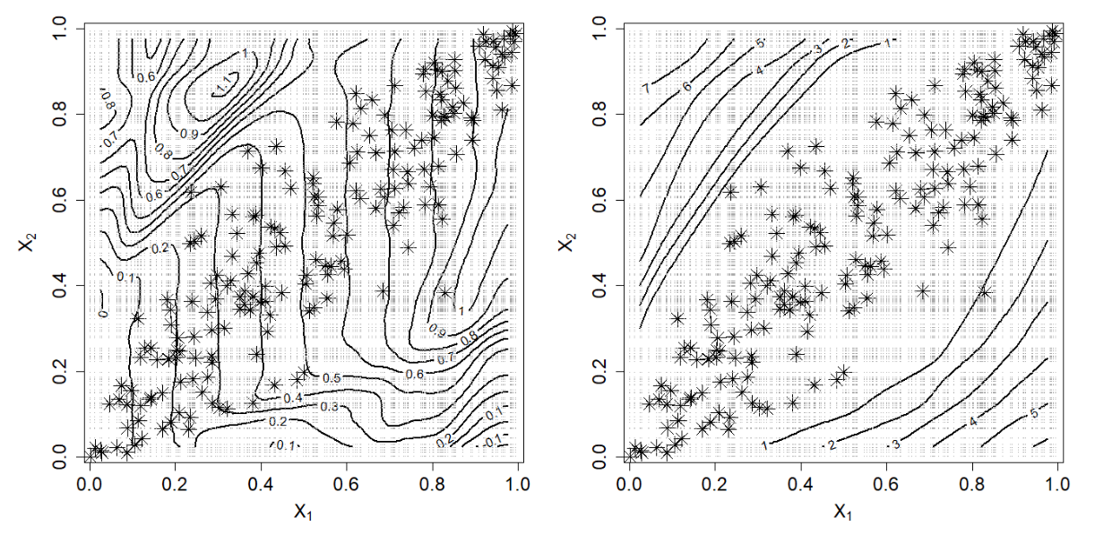
Figure 5 from the paper
For neural networks, the bias can be explained by the very high variance in the extrapolation areas.
Alternatives
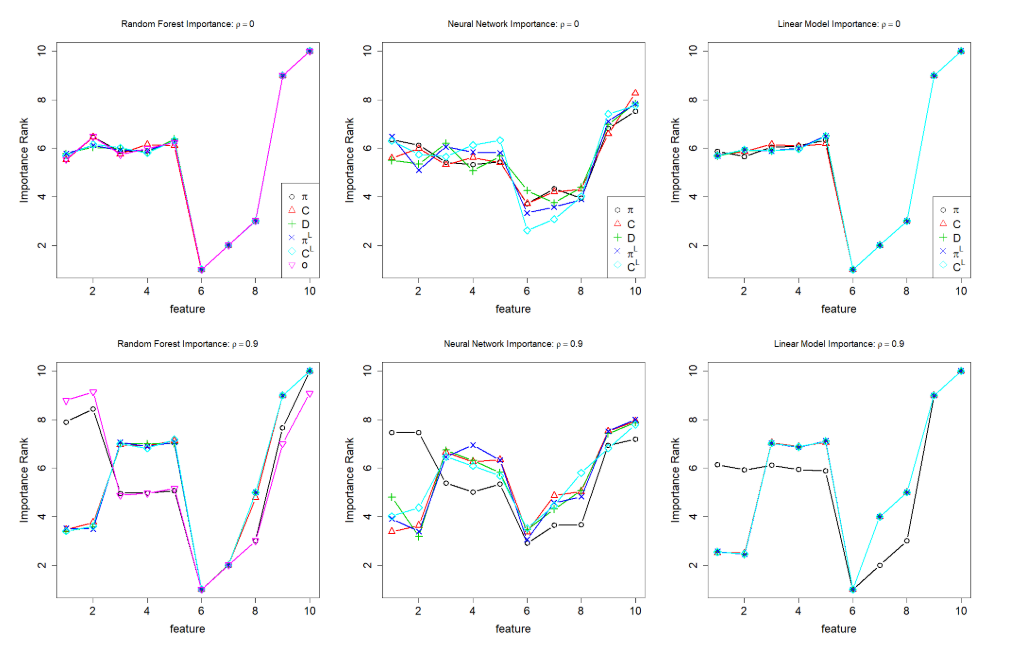
Figure 7 from the paper
The four alternatives described in the TL;DR section all correctly tune down the importance of the first two features when they are significantly correlated, and agrees on the overall ranking of features in this simple linear dataset.
The agreement might not last in nonlinear or more noisy datasets, and each of the four alternatives requires a different amount of computing resources. So you’ll still need to carefully consider your use case and pick one to use. But you can be sure that the any of these four importance measures won’t be heavily biased as the permutation importance.