
As hinted in the previous post “Building a Summary System in Minutes”, I’ll try do some source code analysis of OpenNMT-py project in this post. I’d like to start with its Beam Search implementation. It is widely used in seq2seq models, but I haven’t yet had a good grasp on its details. The translator/predictor of OpenNMT-py is also one of the most powerful I’ve seen, coming with a wide range of parameters and options.
It turned out that writing this post was much harder than I imagined. I found it very hard to succinctly introduce the inner workings of a process while also cover the important code chunks at the same time. Due to this difficulty, the post will be split into at least two pieces, one basic and one advanced, to avoid creating too much distraction along the way.
I feel much more confident in my knowledge of Beam Search after writing this post. I hope you can feel the same after reading it. :)
A Quick Review of Seq2Seq and Beam Search
An seq2seq feed-forward example (source)
A seq2seq (sequence-to-sequence) model maps an input sequence to an output sequence. The input sequence is fed into an encoder, and the hidden state of the encoder (usually at the final time step) is used as the initial hidden states of a decoder, which in turns generates the output sequence one-by-one. Usually the model employs a variation of the attention mechanism, which let the model selectively concentrates on a subset of the input time steps according the decoder states (by using a softmax activation function).
The most straight forward way to generate output sequences is to use a greedy algorithm. Pick the token with the highest probability, and move on to the next. However, it can often lead to sub-optimal output sequences.
One common way to deal with this problem is to use Beam Search. It uses breadth-first search to build its search tree, but only keeps top N (beam size) nodes at each level in memory. The next level will then be expanded from these N nodes. It’s still a greedy algorithm, but a lot less greedy than the previous one as its search space is larger.
The following is an example of beam search of size 5:
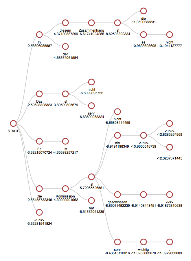
A Beam Search Example (Source)
The number below each node is the log probability of the sequence thus far. The probability of a sequence a_1, a_2, a_3 can be calculated as a conditional probability P(a_1, a_2, a_3) = P(a_1)P(a_2|a_1)P(a_3|a_1, a_2). Take natural log of that and it becomes additive. The search ends when end-of-sentence/end-of-sequence (EOS) token appears as the most possible prediction, and we have a complete sequence generated.
How to Do Beam Search Efficiently
After kick-start the search with N nodes at the first level, the naive way is to run the model N times with each of these nodes as the decoder input. If the maximum length of the output sequence is T, we’ll have to run the model N*T times in the worst case.
The smarter way is to put these N nodes into a batch and feed it to the model. It’ll be much faster since we can parallelize the computation, especially when using a CUDA backend.
We’ll soon see that an even better way is to do multiple beam searches at the same time. If we’re trying to generate output sequences for M input sequences, the effective batch size would become N * M. You’ll need this number to estimate whether the batch will fit into your system memory.
The OpenNMT-py Implementation
How I Find Where to Look
The start point is translate.py (the script for making inferences/predictions), which contains:
translator = build_translator(opt, report_score=True)
translator.translate(src_path=opt.src,
                     tgt_path=opt.tgt,
                     src_dir=opt.src_dir,
                     batch_size=opt.batch_size,
                     attn_debug=opt.attn_debug)
It leads us to onmt/translate/translator.py, which contains the function build_translator and the class Translator. Translator.translate method uses Translator.translate_batch method to generate output sequences (translation) for a batch.
There are two modes of the translate_batch method (fast = True/False). We’ll ignore the fast mode for now as it does not support all features. For fast = False translate_batch will defer to Translator._translate_batch, where most of the magic happens.
Finally, in Translator._translate_batch we see the following statement:
beam = [
    onmt.translate.Beam(beam_size, n_best=self.n_best,
                        cuda=self.cuda,
                        global_scorer=self.global_scorer,
                        pad=vocab.stoi[inputters.PAD_WORD],
                        eos=vocab.stoi[inputters.EOS_WORD],
                        bos=vocab.stoi[inputters.BOS_WORD],
                        min_length=self.min_length,
                        stepwise_penalty=self.stepwise_penalty,
                        block_ngram_repeat=self.block_ngram_repeat,
                        exclusion_tokens=exclusion_tokens)
    for __ in range(batch_size)
]
The statement creates a Beam object for each one of the input sequences. It leads us to the final piece of the puzzle — onmt/translate/beam.py.
(We’re going to ignore some advanced features, such as copy attention, length and coverage penalties for now to simplify things. They will be covered in the next part of this series.)
The Big Picture (_translate_batch method)
For demonstrative purpose, suppose we have a batch of size 3, each with length 4 (can already be padded). The three input sequences are denoted as a, b, and c:
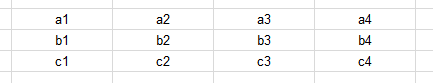
A 3x4 input tensor for the encoder.
The _translate_batch method first feed the input sequences to the encoder, and get the final hidden states and outputs at each time step in return:
src, enc_states, memory_bank, src_lengths = self._run_encoder(
    batch, data_type)
Suppose the model has four encoder hidden states for each sequence/example, and we want to do a beam search with a size of four. The following statement:
self.model.decoder.map_state(\_repeat_beam_size_times)
expands the final encoder hidden states:
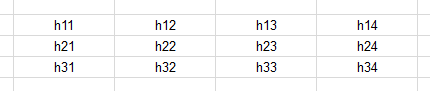
Fig 1: The final encoder hidden states: a 3x4 tensor
to a (3x4)x4 tensor:
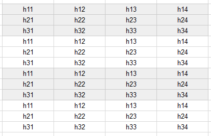
Fig 2: The expanded hidden states: a 12x4 tensor
(This is a simplified example. LSTM actually has two tensors as its hidden states.)
It set up the decoder to run 3x4 sequences at a time (i.e. use a batch size of 12), so we can do beam searches on these three input sequences simultaneously.
Then it enters a loop that runs at most self.max_length times. At the start of each iteration, right after checking the stopping condition, it creates the decoder inputs by collecting the predictions from the last time step (which will be a Beginning-of-Sentence/BOS token if it’s at the first time step):
# Construct batch x beam_size nxt words.
# Get all the pending current beam words and arrange for forward.
inp = var(
    torch.stack([b.get_current_state() for b in beam]
).t().contiguous().view(1, -1))
The above statement is very important, so let’s take closer look. Let the prediction for input sequences (a, b, c) at the previous time step be (A, B, C). The expression torch.stack([b.get_current_state() for b in beam]) creates a 3x4 tensor:
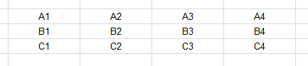
Fig 3: Previous decoder predictions
The .t() operation flips the tensor into a 4x3 one:
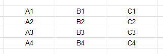
Fig 4: Transposed predictions
Then .view(1, -1) flattens the tensor into a 1x12 one:

Fig 5: Flatten predictions
Note that the sequences are repeated in the same pattern as in Fig 2 for hidden states.
The predictions are then fed into the decoder as inputs:
dec_out, attn = self.model.decoder(inp, memory_bank,
    memory_lengths=memory_lengths,
    step=i)
The decoder outputs are fed into a generator model to get the final (log) probability outputs (self.model.generator.forward). The probabilities are then converted into a 4x3x(num_words) tensor (with and without copy-attention mechanism).
For each input sequence, the corresponding (log) probability outputs are passed to its Beam object (b.advance):
for j, b in enumerate(beam):
    b.advance(out[:, j],
        beam_attn.data[:, j, :memory_lengths[j]])
    select_indices_array.append(
b.get_current_origin() \* batch_size + j)
The list select_indices_array records the nodes on which the Beam object has expanded.
b.get_current_origin() returns the local indices of the nodes (the number part minus 1 in Fig 5). And b.get_current_origin() * batch_size + j recovers its corresponding position in the decoder input (expanded batch). For example, for the second input sequence (j=1), if the beam selected the second node to expand, the formula would be evaluated as (2–1) * 3 + 1= 4, which points to B2 in Fig 5.
The list select_indices_array is then collated into a 3x4 tensor, flipped, and finally flatten, just like in Fig 3–5.
Because it’s possible that only some of the nodes are expanded, and the order of node can be changed, we need to re-align the hidden state of the decoder for the next time step using select_indices_array:
self.model.decoder.map_state(
    lambda state, dim: state.index_select(dim, select_indices))
As an example, consider this set of hidden states of a decoder (the final index is the node index):
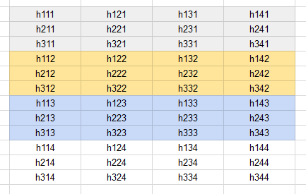
Fig 6: The hidden states of the decoder right after the feed-forward ops
Suppose the first sequence expanded on node [1, 3, 2, 1], the second on [2, 3, 1, 2], the third on [1, 2, 3, 4], then the re-aligned hidden states would be:
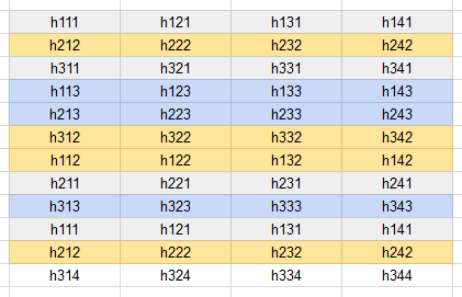
Fig 7: Re-aligned hidden states of the decoder
After the stopping condition has been met, the method collect the final predictions from each Beam object (and also the attention vectors), and return the results to the caller:
ret = self.\_from_beam(beam)
What Happens inside a Beam object?
The two most important instance variables are next_ys and prev_ks, retrievable by invoking .get_current_state and .get_current_origin methods, respectively. The top (beam_size) predictions for the next decoder output at each time step are stored in next_ys(they are the nodes in the search tree). Information about which nodes from the previous step have the next_ys been based on is stored in prev_ks. They are both required to reconstruct the output sequence from the search tree.
Most of the operations are done inside the method .advance. It takes the (log) probability outputs and attention vectors from the generator (which takes the output from the decoder) as arguments.
If the decoder is not at the first time step, then the method sums up the (log) probability outputs with the previous scores, which are also log probabilities. It represents the probability of the output sequence (remember that log probabilities are additive):
beam_scores = word_probs + \
    self.scores.unsqueeze(1).expand_as(word_probs)
Suppose in our example we have a target vocabulary with a size of 10000, then beam_scores would be a 4x10000 tensor. It represents 40000 possible sequences and their (log) probabilities of occurence.
The method then makes sure that it doesn’t expand on EOS nodes by setting the probabilities of the sequences that expand on the nodes to be a very small value:
for i in range(self.next_ys[-1].size(0)):
    if self.next_ys[-1][i] == self._eos:
        beam_scores[i] = -1e20
The scores/probabilities tensor is flattened, and topk method is used to extract the most possible (beam_size) sequences. They are the new nodes to be added to the search tree:
flat_beam_scores = beam_scores.view(-1)
best_scores, best_scores_id = flat_beam_scores.topk(self.size, 0,
    True, True)
The method needs to recover the node indices and token indices from best_score_id, in order to update prev_ks and next_ys, respectively:
# best_scores_id is flattened beam x word array, so calculate which
# word and beam each score came from
prev_k = best_scores_id / num_words
self.prev_ks.append(prev_k)
self.next_ys.append((best_scores_id - prev_k * num_words))
(20181106 Update: I forgot to mention how the method deal with EOS tokens at the end of the sequences. Added a paragraph below to fix this.)
Now the method examines these new nodes to see if any of them is an EOS token (which completes the output sequence). If so, the sequence is added to a list self.finished as output candidates:
for i in range(self.next_ys[-1].size(0)):
    if self.next_ys[-1][i] == self._eos:
        global_scores = self.global_scorer.score(self, self.scores)
        s = global_scores[i]
        self.finished.append((s, len(self.next_ys) - 1, i))
Finally, it checks the stopping condition (if an EOS token is at the end of the most possible sequence) and set the eos_top flag:
# End condition is when top-of-beam is EOS and no global score.
if self.next_ys[-1][0] == self._eos:
    self.all_scores.append(self.scores)
    self.eos_top = True
That’s it! We’ve covered the whole beam search process (admittedly, omitted a few details and advanced features).
One last interesting thing I’ll add is the Beam.get_hyp method, which reconstructs an output sequence ending at kth node at time timestep (if you consider the BOS token is located at time step 0)(it does not return BOS):
def get_hyp(self, timestep, k):
    """
    Walk back to construct the full hypothesis.
    """
    hyp, attn = [], []
    for j in range(len(self.prev_ks[:timestep]) - 1, -1, -1):
        hyp.append(self.next_ys[j + 1][k])
        attn.append(self.attn[j][k])
        k = self.prev_ks[j][k]
    return hyp[::-1], torch.stack(attn[::-1])
To Be Continued…
Thanks for reading!
I’ll try to cover the more advanced features I intentionally left out here in the next part.